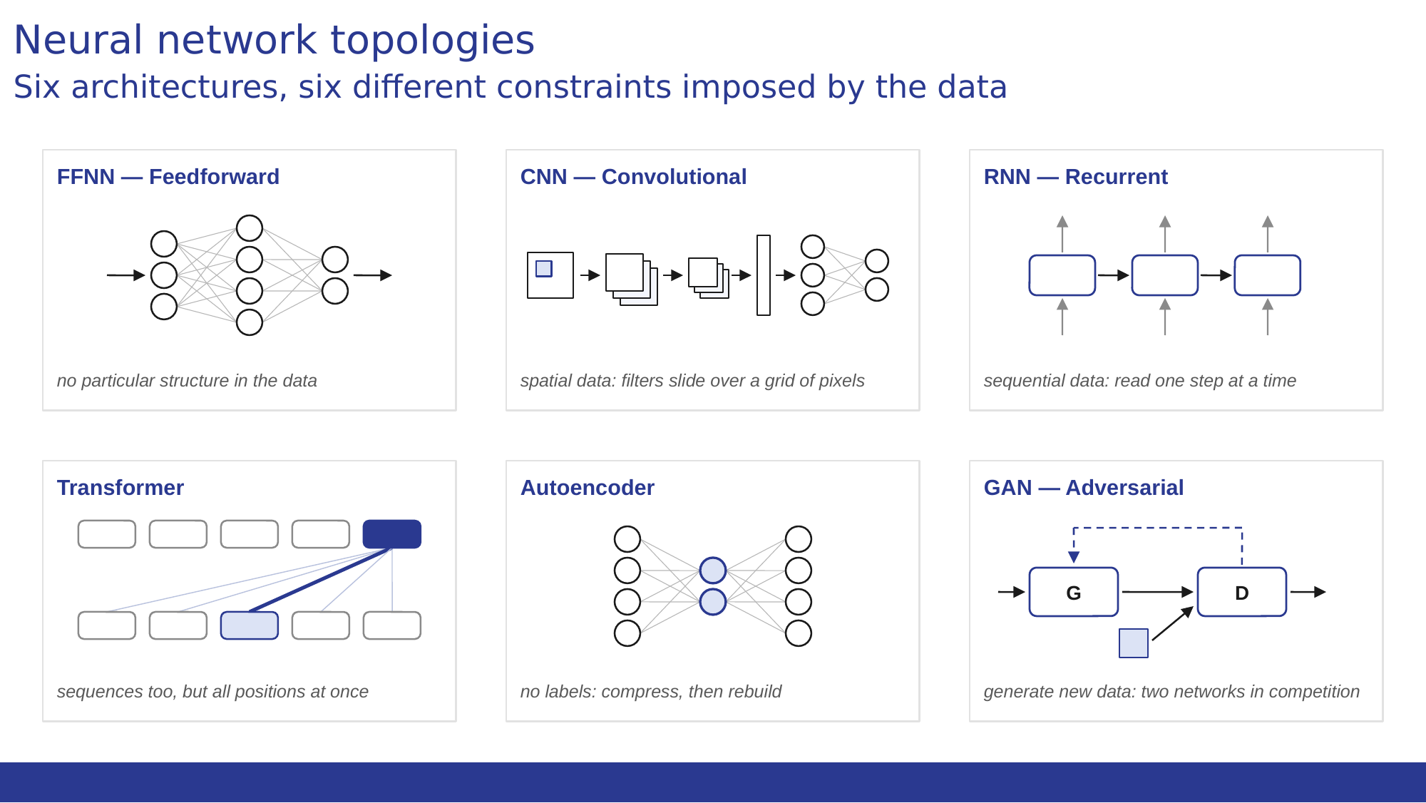
In chapter 6 we said that the network described there, where information flows only forward and every node in a layer is connected to all the nodes in the next one — a feedforward, fully connected network — is only one of the possible topologies, and we put the others off until this chapter. In chapter 9 we closed the circle again, recalling that it was only one of the possible topologies. It is time to keep that promise.
Every architecture we are about to see was born to answer a different constraint imposed by the data: an image has a spatial structure, a sentence has an order that matters, and sometimes you don’t even want to predict a label but to generate something new that did not exist before. We will look at five families, each built around a simple idea that answers one of those constraints.
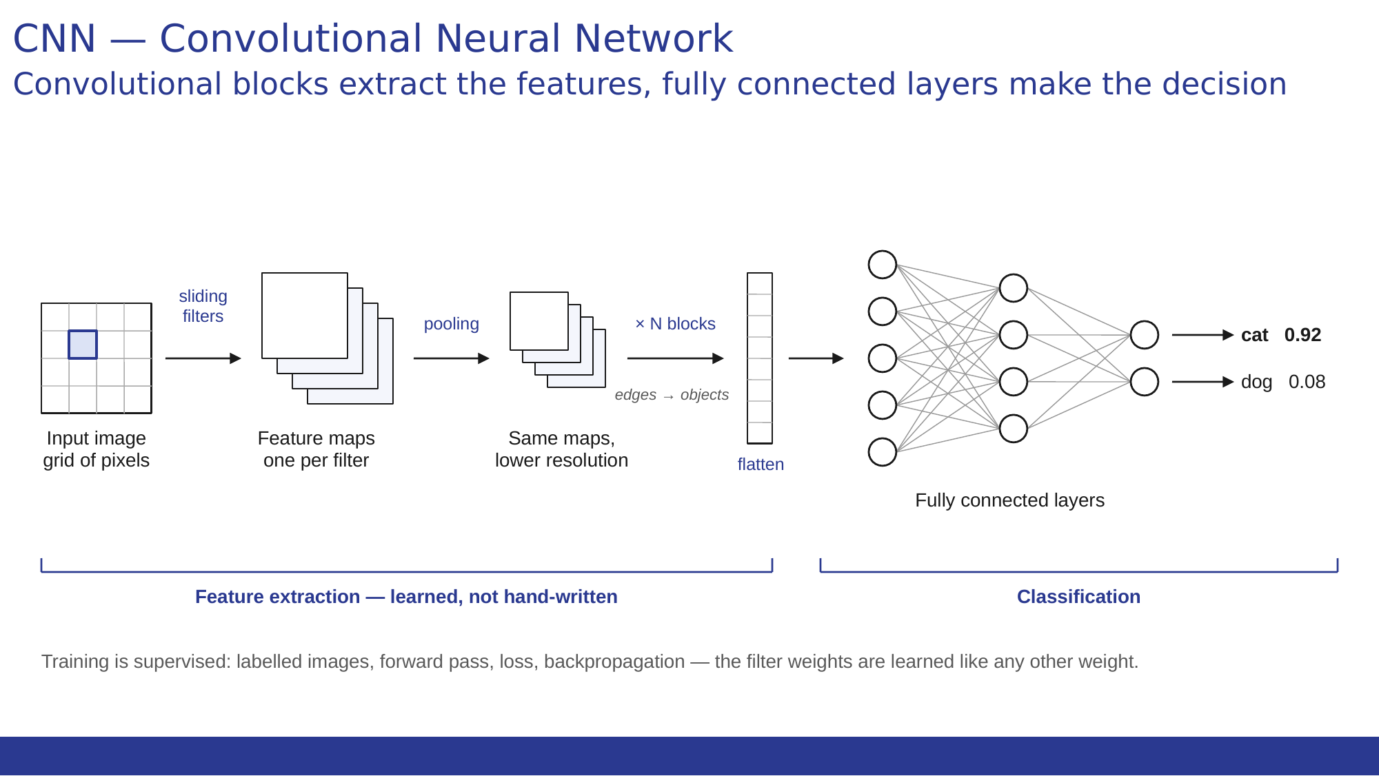
CNN, Convolutional Neural Network. It was born to work on images, that is, on data organized in a spatial grid of pixels. The name comes from the central operation itself: small filters are slid — convolved — across the image, and each filter learns to recognize a local feature, an edge, a texture, a curve, without anyone telling it in advance what to look for. Many filters are applied to the same image in parallel, dozens or hundreds, and each produces a map of its own, so that from one image you obtain as many maps as there are filters, one for every feature detected. A pooling layer then compresses the spatial resolution of each map, keeping only the strongest signal in each neighborhood and discarding the exact position where it sat: the feature survives, but the network becomes less sensitive to small shifts. By stacking several blocks of this kind, the later layers combine the simpler features into progressively more complex shapes, from edges to whole objects.
After several blocks of filtering and pooling, the feature maps are flattened into a single vector and passed to one or more fully connected layers, exactly like those seen in the previous chapters, which combine all the extracted features to produce the final output — for example, the probability that the image contains a cat rather than a dog. In a sense, the convolutional part does the job of finding the right features, and the final fully connected part does the job of deciding on the basis of those features.
Training is supervised: the network is given labeled images, and forward pass, loss, and backpropagation adjust the weights, including those inside each filter. No human writes the filters: it is training that decides on its own, example after example, which features are worth extracting in order to distinguish, say, a cat from a dog. The main domain remains computer vision: image recognition, object detection, medical imaging.
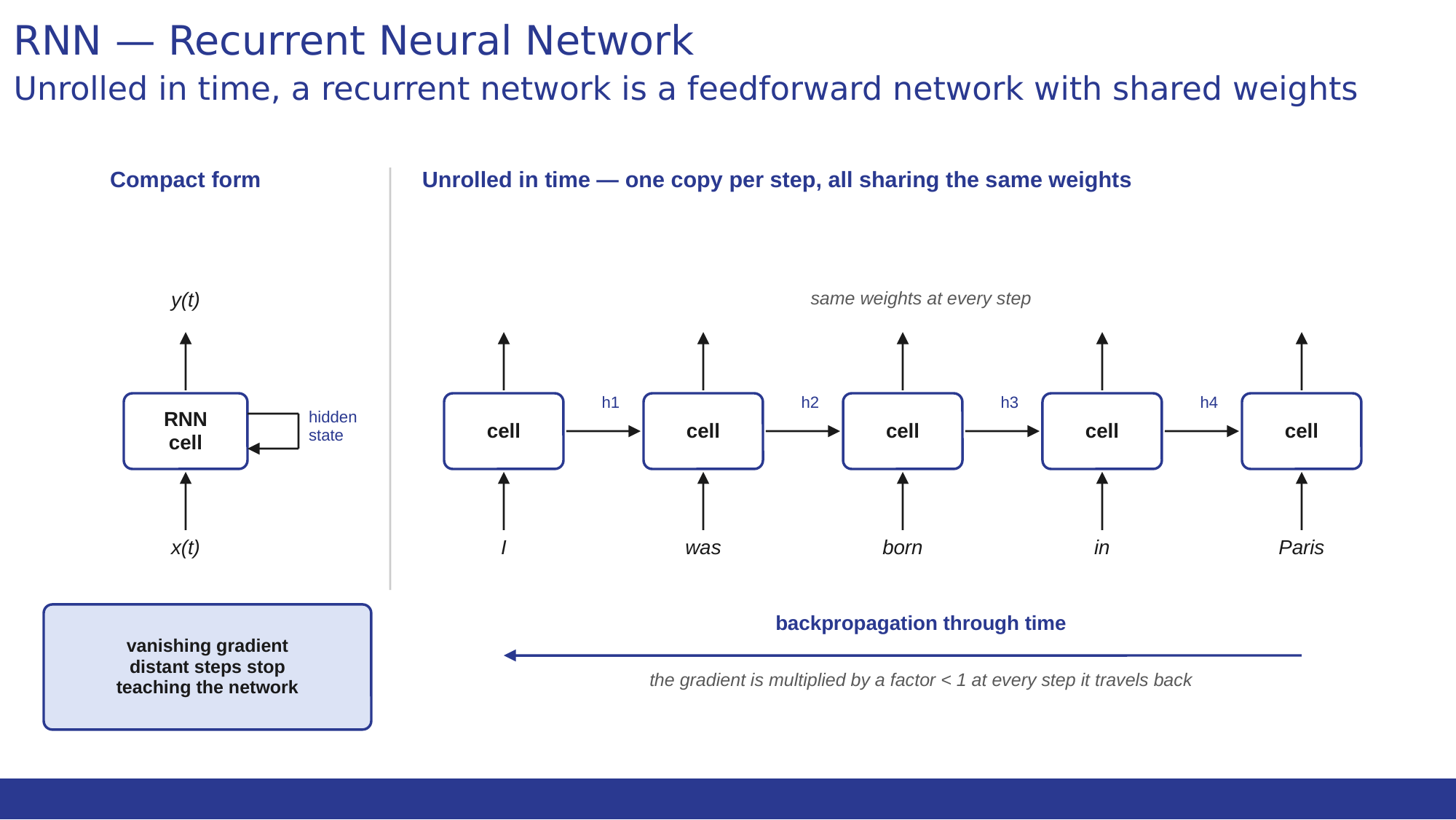
RNN, Recurrent Neural Network. It was born for the opposite problem to the CNN: sequential data, where order matters, such as text or time series. The key idea is the feedback loop: unlike a feedforward network, where information flows only forward, in an RNN the network holds an internal state that at each step feeds back and is given to it again together with the next element of the sequence. That state that feeds back is called the hidden state, and it is distinct from the output proper, which at each step is derived from it: because the hidden state depends on the current word and on the hidden state of the previous step, which in turn depended on the word before that, and so on backward, it ends up being a function of every word read so far.
To see how it is trained, it helps to imagine unrolling the network in time: instead of a single cell calling itself, you redraw it as a feedforward network with as many layers as there are steps in the sequence, each one a copy of the same cell, receiving as input the word for that instant together with the hidden state of the previous layer. Seen this way, the RNN is simply a feedforward network with the weights shared across all the layers, and training uses exactly the same backpropagation as in chapter 8, except the layers have become moments in time: hence the name backpropagation through time.
And this is precisely where the main limitation arises. At every layer it crosses on its way back, the gradient gets multiplied by a factor typically smaller than one, and multiplying many numbers smaller than one together, after a few dozen steps the gradient shrinks to practically nothing: the network stops learning from information far in the past, and its behavior ends up depending almost entirely on the last few elements of the sequence. This is because the update to the weights is the sum of the contributions arriving from every step of the sequence: if the contribution tied to a distant piece of information is practically zero, the weights keep updating, but only on the basis of what happened in the last few steps. Distant dependencies, quite simply, stop teaching the network anything. This is the so-called vanishing gradient problem, and variants such as LSTM, Long Short-Term Memory, and GRU, Gated Recurrent Unit, were born precisely to mitigate it: instead of overwriting the whole hidden state at every step, they introduce gates that explicitly decide what to keep and what to discard from the previous information, so that the relevant signal can travel across many steps without fading away*. And it is exactly this structural limitation that opens the way to the next chapter.
*The gates are not hand-written rules; they are themselves small layers with their own weights, learned during training with the same backpropagation through time.
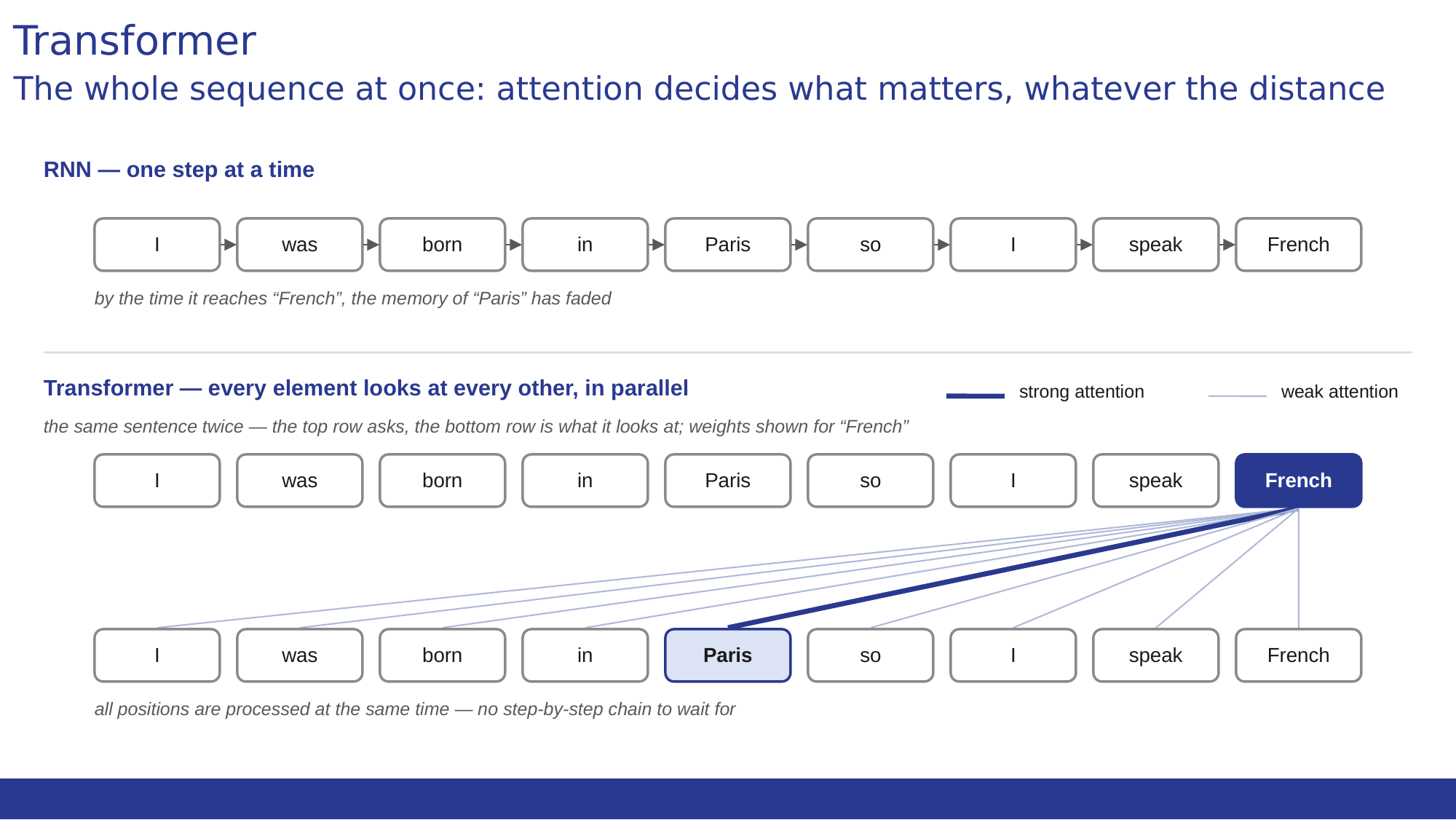
Transformer. It was born precisely to overcome the RNN’s bottleneck: reading one element at a time. Instead of scanning the sentence word after word, carrying along a summary that decays with distance, the Transformer looks at all the positions at once and, for every word, computes how much each of the others matters in order to interpret it. This is the mechanism called attention.
The gain is twofold. First: a distant dependency is no longer a long chain to climb back through. If the word French depends on the word Paris, a few positions earlier, attention connects them directly, in a single step, and the vanishing gradient problem does not arise in the same form. Second, and this is what changed the history of the field: computing all the positions together is an operation a GPU can parallelize massively, so training scales to quantities of text that would have been unthinkable for a recurrent network.
It is the architecture on which practically every large language model in use today is built, and it is the subject of Series 4, where we will open it up and look at it component by component. For now one sentence will do: the Transformer reads sequences too, but all at once rather than one step at a time.
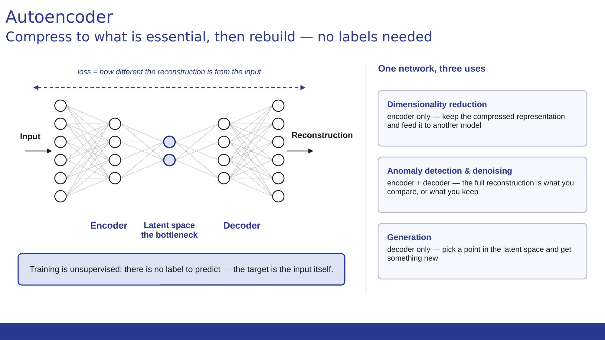
Autoencoder. This is a network born for unsupervised learning, and its structure is distinctive: it compresses the input into a low-dimensional representation, called the latent space or bottleneck, and then tries to reconstruct the original input from that compressed representation. The first half, which compresses, is called the encoder; the second, which reconstructs, the decoder. In chapter 9 we met the sparse autoencoder, which did the opposite — it expanded a few overcrowded dimensions into a wider space to make the features more legible: here the central operation is the original one, compress and then rebuild.
Since there are no labels, the training objective is simply that the reconstructed output should be as close as possible to the original input: the loss measures the difference between the two. Precisely because the network is forced to pass through that bottleneck, it is obliged to learn which features of the input are genuinely essential in order to rebuild it, discarding the noise.
Once trained, the encoder and the decoder can also be separated and used on their own. The decoder alone becomes a generator: starting from a point in the latent space, it produces a new output. In a plain autoencoder this only works up to a point, because the latent space is not organized for it and a point picked at random may rebuild into something that means nothing: it is variational autoencoders that fix exactly this, and it is from there that the idea connects to the wider family of generative models.
The main domains, accordingly, divide by which of the two halves they use. In dimensionality reduction only the encoder is used: all that is needed is the compressed representation — for instance, the few dimensions that summarize hundreds of features of a customer, to be passed on to another model such as a recommendation system. In anomaly detection and denoising, by contrast, encoder and decoder are used together, because in both cases the full reconstruction is needed: in the first, to compare it against the original input, as in credit card transaction monitoring, where an anomalous input reconstructs worse than a normal one; in the second, to return a clean version of the noisy input, as in medical imaging, where the autoencoder learns to give back a sharper scan.
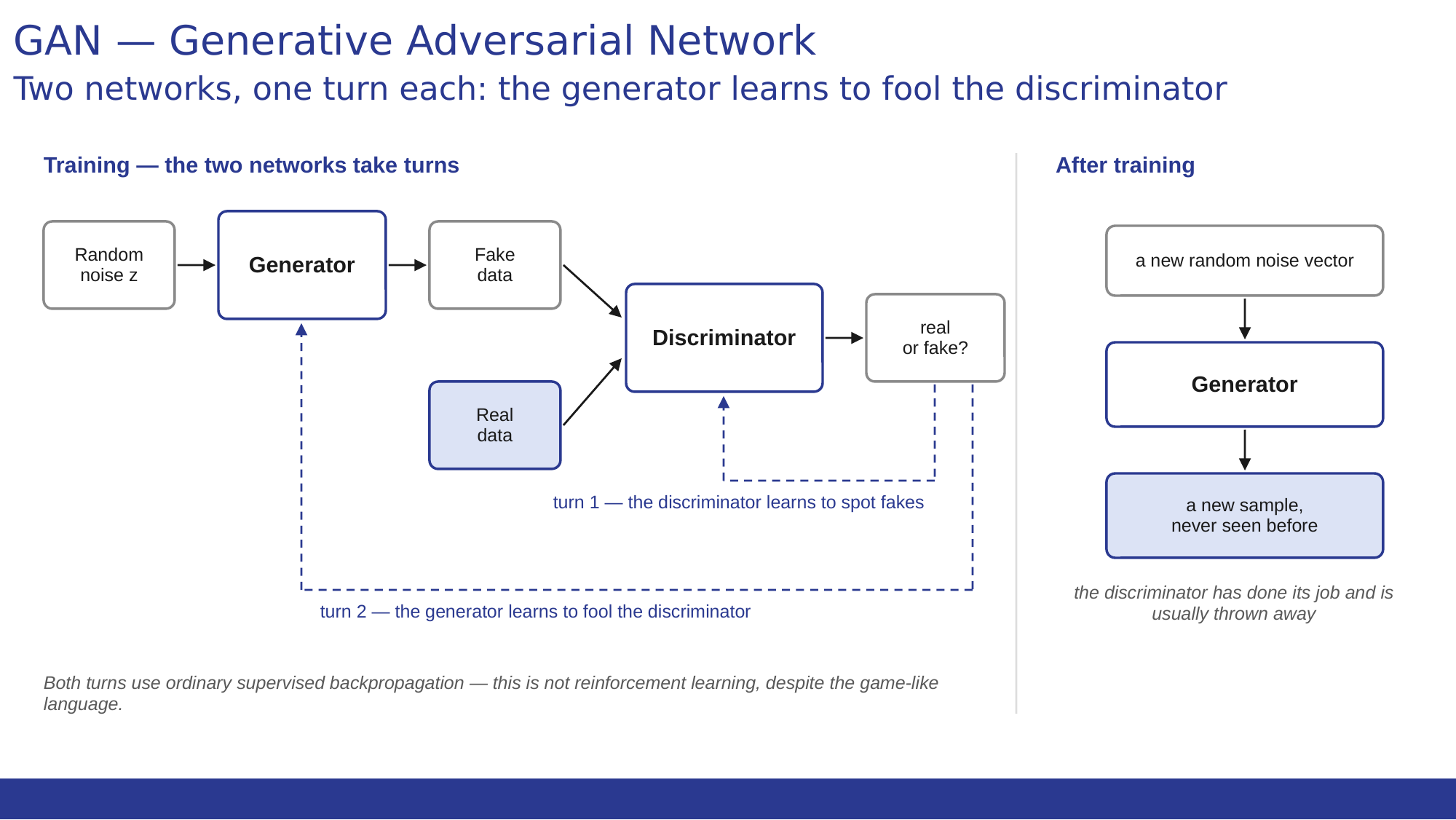
GAN, Generative Adversarial Network. It is made of two distinct networks trained against each other: the generator and the discriminator. The generator starts from random noise and tries to produce fake data that looks real, for example images; the discriminator receives both real data and the fake data produced by the generator, and has to learn to tell them apart.
Training proceeds in turns. In each cycle, the discriminator is trained first: it is shown real examples, labeled as genuine, and examples freshly produced by the generator, labeled as fake, and its weights are adjusted with ordinary backpropagation so that it learns to recognize them. Then the generator is trained: it produces new fake data, which is passed to the discriminator, but this time the generator’s loss measures how well it managed to pass them off as real, so its weights are adjusted in the direction that maximizes the discriminator’s error. The two networks therefore play a more or less zero-sum game, until the generator becomes capable of producing data practically indistinguishable from the real thing.
One clarification is worth making: this scheme of two agents in competition is reminiscent in some ways of the reinforcement learning of chapter 5, and it is no accident that it is often described in similar language — zero-sum game, equilibrium, strategy. But from the algorithm’s point of view it remains supervised learning applied twice: both generator and discriminator are updated with ordinary backpropagation on a differentiable loss, not with rewards and a policy.
Once training is complete, it is almost always only the generator that gets used: you feed it a new vector of random noise, different every time, and it returns a new image, never seen before, consistent with the style of the data it was trained on. The discriminator is normally discarded, and only finds use in specific contexts, such as synthetic content detection. In its basic form, moreover, you cannot ask the generator for anything specific: every output arises from a point chosen at random in the noise space. Variants designed precisely for this exist, such as conditional GANs, where the noise is accompanied by a control label seen by both networks during training.
The main domains are the generation of realistic images and video, style transfer, and the artificial augmentation of datasets when real data is scarce. With the arrival of diffusion models, which we will discuss in chapter 30, GANs have lost ground in text-to-image generation, but they remain competitive in niches where speed and computational cost matter, such as upscaling or real-time style transfer.
With these five families the catalog of basic architectures is complete, and with it Series 2. One constraint remains, though, one we have already met and never really resolved: a neural network, whatever its topology, speaks only the language of numbers. If I want a CNN to see an image or a Transformer to read a sentence, that image and that sentence must first become numbers — and not just any numbers: numbers that carry meaning with them. That is the question the next series opens with: can a number really mean something?