
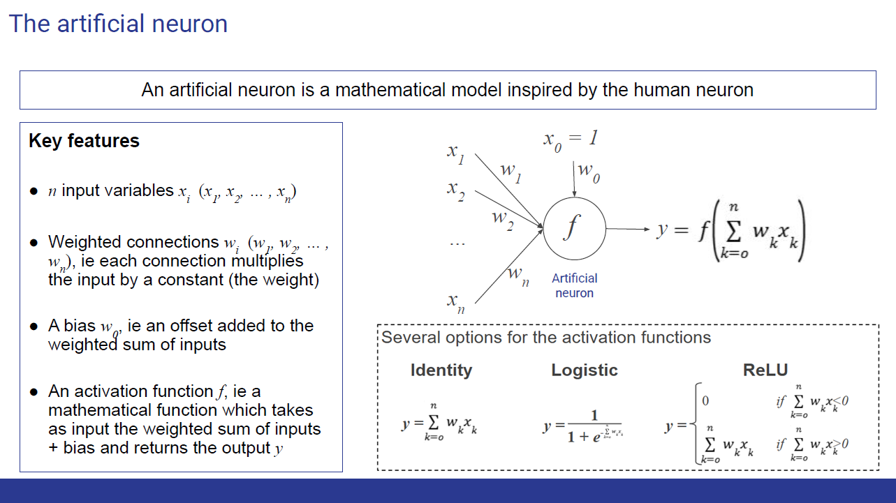
In the previous chapter we said that a network is made of elementary nodes, and that by combining enough of them you can, at least in principle, represent any relationship between input and output. But we left the promise half-kept: what, exactly, does one of those nodes do? And how do the formulas arise when you put them together? Let’s look inside a node.
What a neuron computes. An artificial neuron is a small mathematical model with four ingredients:
- the inputs — n incoming numbers, x₁, x₂, …, xₙ, arriving from the nodes of the previous layer (or, for the first layer, directly from the data);
- the weighted connections — each input is multiplied by its own weight w₁, w₂, …, wₙ, and the products are summed. It is the same weighted sum as in chapter 3, now seen from inside a single node;
- the bias — a term w₀ added to the weighted sum, an offset that shifts the threshold at which the neuron activates, independently of the inputs;
- the activation function — a function f that takes the weighted sum plus the bias and returns the neuron’s output y.
In one line: multiply each input by its weight, add everything up, add the bias, and pass the result through f. That’s all.
Activation functions. The choice of f changes the neuron’s character. Three typical examples:
- the identity — the output equals the weighted sum, with no transformation at all. Simple, but, as we’ll see shortly, with a fatal flaw;
- the logistic (or sigmoid) — squashes any value into a number between 0 and 1, useful when the output is to be read as a probability;
- the ReLU — lets positive values through unchanged and zeroes out negative ones. In its GELU variant, which smooths the sharp corner around zero, replacing it with a soft transition, it has long been, and still is, one of the most widely used activation functions in deep networks.
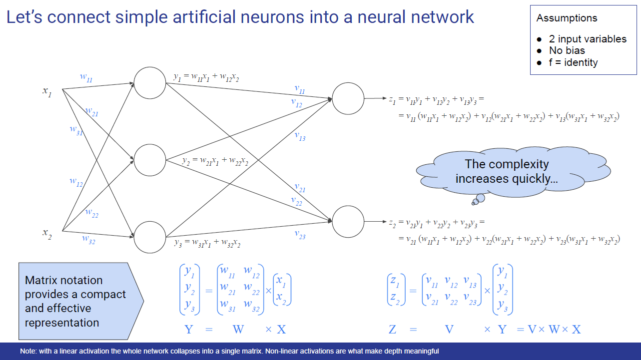
How combined neurons produce the formulas. Take a small example network: two inputs, a hidden layer of three neurons, two output neurons (the bias is left out of the example, to keep the formulas light). Each hidden neuron computes its own weighted sum of the inputs; each output neuron computes its own weighted sum of the hidden outputs. Written out in full, these expressions quickly become very complex, which is why matrix notation is used: the outputs of a layer are obtained by multiplying a matrix of weights by the vector of inputs, and the entire two-layer network is written, very compactly, as Z = V × W × X.
And here the activation function returns, with a role that is anything but decorative. If f is the identity — that is, if there is no non-linearity — that product of matrices can be multiplied out once and for all and reduced to a single matrix. In other words: a deep network with linear activation collapses into a single layer, and all the depth we spoke of in chapter 6 vanishes. It is the non-linearity of the activation function that prevents this collapse — it is what makes depth truly meaningful. Without it, a thousand layers would be worth no more than one.
That is why a neuron is not just “weighted sum plus bias”: that small non-linear piece at the end is what gives a deep network its real power. In the next chapter we’ll see how the millions of weights we’ve introduced are found, all together: backpropagation.