In chapter 3 we said that training a model means finding the weights that make the loss as small as possible, and that gradient descent walks down the loss surface toward a minimum. But we left a question hanging: in which direction should the step be taken? Answering that question is all that backpropagation does.
Where the minimum lies. Let us start from the way a minimum is found at school. Given a function, its minimum point sits where the first derivative vanishes: at the lowest point the curve is momentarily flat, the slope is zero. For our loss the principle is identical, with one complication: the loss does not depend on a single variable but on all the weights of the model. Instead of a single derivative we therefore have a partial derivative of the loss with respect to each weight — how much the loss would change if we moved that weight while keeping all the others fixed. The vector collecting all these partial derivatives is called the gradient.
The gradient is not just a list of numbers: it has a precise geometric meaning. At every point of the loss surface it points in the direction of steepest ascent — the direction along which the loss grows fastest. And here the circle closes with chapter 3: if the gradient tells us where the climb is steepest, then to descend we simply go in the opposite direction. That is exactly what gradient descent does. The minimum, for its part, sits where the gradient vanishes: where there is no longer any direction in which to descend.
Why we do not solve, we descend. It would be tempting to do what we did at school: set the gradient to zero and solve the system. On a real model this is impossible. Such a system would have millions — today billions — of equations, one per weight, almost all of them non-linear and tangled together: no closed-form formula solves it. This is why we give up on solving and fall back on descending: gradient descent does not find the minimum in a single move, it gets there in small steps. But every step still requires the gradient at that point — the derivative of the loss with respect to every single weight. How do we compute millions of derivatives efficiently? This is where backpropagation comes in.
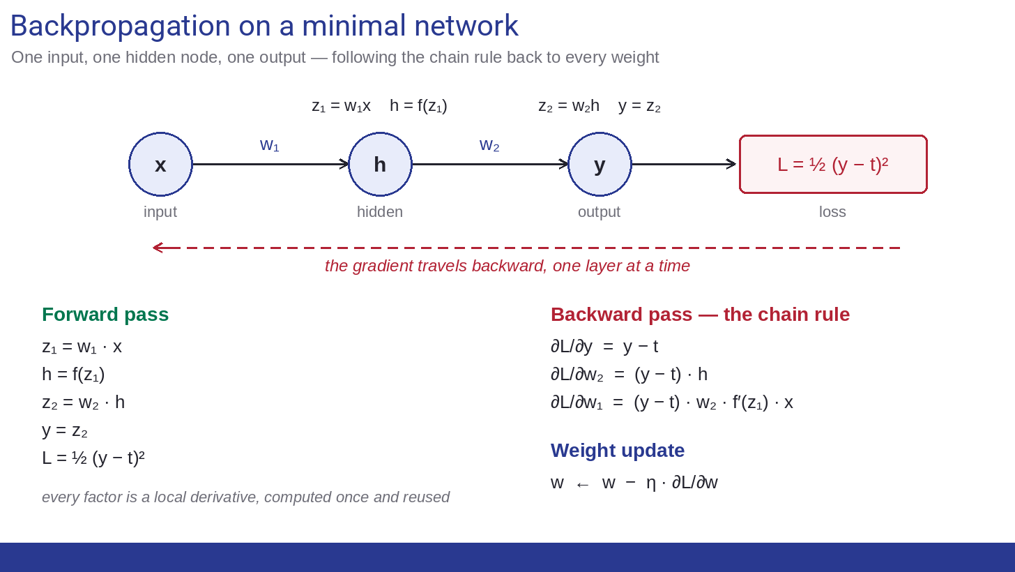
The chain rule. Look at the minimal network in the diagram: the input x enters the hidden node through the weight w₁, comes out transformed into h, travels through the weight w₂ to the output y, and from y the loss L is computed. The loss does not depend on w₁ directly: it depends on y, which depends on h, which depends on w₁. It is a chain of dependencies.
And for chains there is a precise rule, the chain rule: the derivative of a composite function is the product of the derivatives of the individual links. The derivative of the loss with respect to w₁ therefore breaks down into a product of local factors — ∂L/∂y · ∂y/∂h · ∂h/∂w₁ — each one simple to compute on its own.
The calculations, spelled out. With the loss L = ½ (y − t)², the first factor is the simplest of all: ∂L/∂y = y − t, the raw error, the distance between what the network predicted and what it should have predicted. From there we climb back up:
- ∂L/∂w₂ = (y − t) · h — the error multiplied by the value that entered w₂;
- ∂L/∂w₁ = (y − t) · w₂ · f′(z₁) · x — the same error multiplied by w₂, by the local derivative of the hidden node, and by the input x.
One factor for every link in the chain, exactly as promised. And note one thing: (y − t), the error at the output, appears in both formulas. It is the signal that propagates backward, and every weight receives a share of it — its own slice of responsibility for the overall error. The more a weight contributed to the mistake, the larger its derivative, and the more decisive its adjustment.
Why every layer can work on its own. Look again at the chain factors for w₁: one of them — ∂L/∂y — is exactly the factor that was also needed for w₂. This is no coincidence. As we climb back up through the network, each layer reuses the work already done by the layer downstream: the derivative of the loss with respect to a layer’s output is obtained from that of the following layer, multiplied by a local derivative — one that concerns only that layer, describing how much its output changes as its input or its weight changes.
And this is what makes the computation tractable. No layer has to redo the calculations starting from the loss: it only needs to receive a single number from the layer downstream — how sensitive the loss is to its output — and combine it with its own local derivatives, which depend only on what it computed itself. In this sense every layer works by looking solely at itself and at the message arriving from downstream, without having to know the whole network.
The two passes. Concretely, the algorithm makes two passes over the network. First a forward pass, in which the input travels through the network up to the loss, and the intermediate values are recorded along the way: z₁, h, z₂, y. Then a backward pass, which starts from the loss and climbs back layer by layer, propagating that sensitivity number and multiplying it, each time, by the local derivatives. Every useful value is computed once and reused on the way back, instead of being recomputed from scratch for every weight. This is where the name comes from: the error propagates backward through the network.
And the training set? So far we have reasoned about a single example — one x, one t — but the real loss, as in chapter 3, is the sum of the errors over all the examples in the training set. The step is straightforward: the gradient of the total loss is the sum of the gradients computed on each example. So we perform a forward and a backward pass for every example, sum the contributions, and only then update the weights. A step of this kind — one that looks at the entire training set before moving — is called a batch.
There is a practical problem, though: if the training set has millions of examples, waiting until all of them have been seen in order to take one single step is painfully slow. In practice we settle on a middle way: the training set is divided into small groups, the mini-batches — a few dozen or a few hundred examples — the gradient is computed on a mini-batch and a step is taken immediately. Then the next mini-batch, and so on. Every step uses only an approximate estimate of the true gradient, but a great many more steps are taken: a trade-off that converges much faster. This is what is known as stochastic gradient descent, and it is how almost all real networks are trained.
The update. At this point we have everything. For every weight: w ← w − η · ∂L/∂w. That η — the learning rate — is the length of the step: make it small and the descent is slow but stable, make it large and we risk overshooting the minimum. One forward pass, one backward pass, one adjustment of all the weights: repeated millions of times, this is the whole training of a neural network.
And it is also the root of its opacity. Backpropagation finds weights that work, but it tells us nothing about what each one means. What remains, in the end, is billions of numbers, tuned to perfection, that nobody wrote and nobody can really read — and that is precisely where the next chapter begins.