
Chapter 11 closed on an open question: in reality, the meaning attached to the dimensions of a dense space is not defined in advance, but learned during training. It’s time to see how.
Before Word2Vec, a fairly natural way to build dense representations was to count: you scan a large text corpus and note, for every word, how many times it appears near every other word. The result is a co-occurrence matrix, in which a word’s row is already, in a sense, a vector describing its behavior in the text. That matrix, though, quickly becomes unmanageable as the vocabulary grows, and has to be reduced with further techniques to become a workable dense space. It also works poorly on words like articles and conjunctions, which appear near vast numbers of different words and end up resembling everything and nothing at once.
Behind the counting of co-occurrences, and behind Word2Vec, lies the same underlying idea, formulated by the linguist John Firth in 1957: you shall know a word by the company it keeps. Two words that often appear in the same contexts tend to have similar meanings. It’s an elegant hypothesis because it turns a problem that seemed to require an understanding of meaning into a far more tractable one: looking at which words sit near which others.
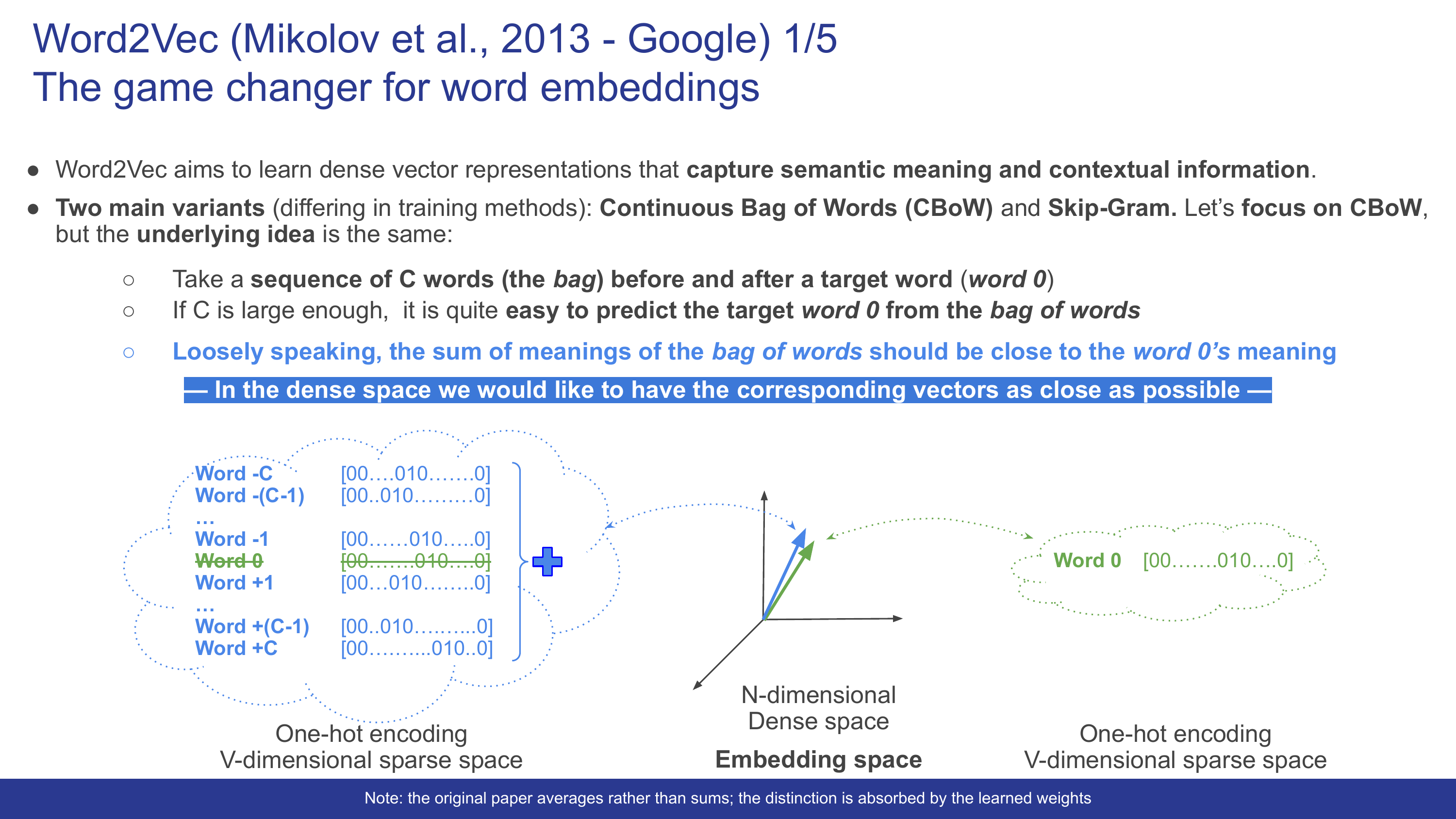
Word2Vec, proposed by Mikolov and colleagues in a 2013 paper out of Google, Efficient Estimation of Word Representations in Vector Space, takes this idea and turns it into an actual training task, solvable with a neural network. There are two complementary variants, differing only in how the prediction task is set up: continuous bag of words, or CBOW, and skip-gram. We’ll focus here on the first, though the underlying idea is the same for both.
The idea behind continuous bag of words is intuitive in its own way, and comes from everyday experience: if you take any text and look at a long enough window of it, and erase the word at the center of a sequence of C words before and C words after, it’s fairly easy to guess the missing word. This idea gives rise to the prediction task: given a sequence of 2C + 1 words — the C words before the target word and the C words after — guess the missing word. Loosely speaking, the goal is to build a space in which the sum of the vector representations of the context words, the C before and the C after, ends up as close as possible to the vector representation of the target word. (The original paper, strictly speaking, averages rather than sums: it’s a difference the learned weights absorb on their own.)
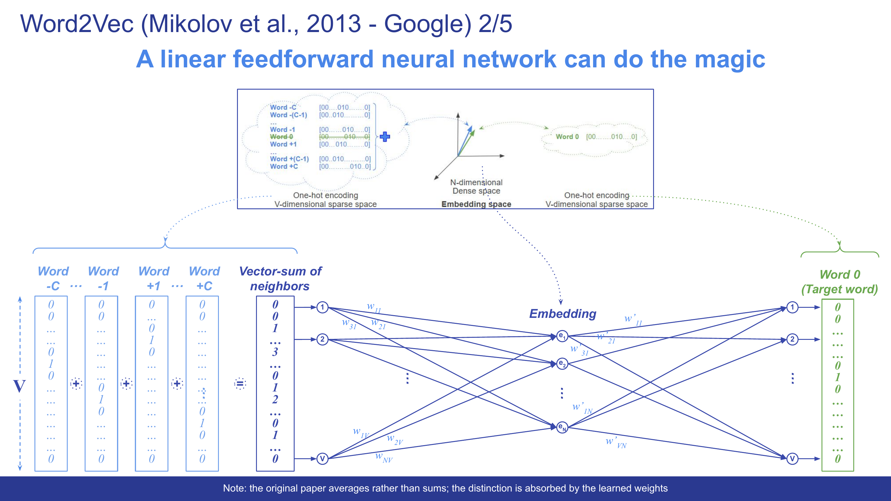
That task can be solved with a very simple feedforward network, with a single hidden layer: an input layer, receiving the sum of the context vectors; a hidden layer, much smaller than the vocabulary; an output layer, as wide again as the vocabulary, that assigns a score to every word: training pushes it to resemble the one-hot vector of the target word as closely as possible. The shape is the hourglass shape of the autoencoder from chapter 10 — wide input, narrow bottleneck, wide output again — and in a sense the objective echoes that of an autoencoder too: we want the final output to resemble, as closely as possible, a representation consistent with the input, even though here the input is the sum of the contexts and the output is the target word, not the very same object. It isn’t an autoencoder in the technical sense, like the one in chapter 10, but it shares both its shape and its spirit. Exactly as in chapter 7, each layer is a weighted sum passing through a matrix of parameters: matrix W connects the input and the hidden layer, matrix W’ connects the hidden layer and the output. With one important difference, though: there is no activation function here, the network is deliberately linear, and so — as we saw in chapter 7 itself — the two matrices could be multiplied out once and for all and reduced to a single one. That isn’t a flaw: here the work isn’t done by depth, it’s done by the bottleneck. The hidden layer is much smaller than the vocabulary and forces everything through a handful of dimensions; it’s that forced compression that produces the embedding. The size of that hidden layer is, in effect, the size of the dense space we’re building, and it’s a size we choose ourselves, not something the model decides on its own.
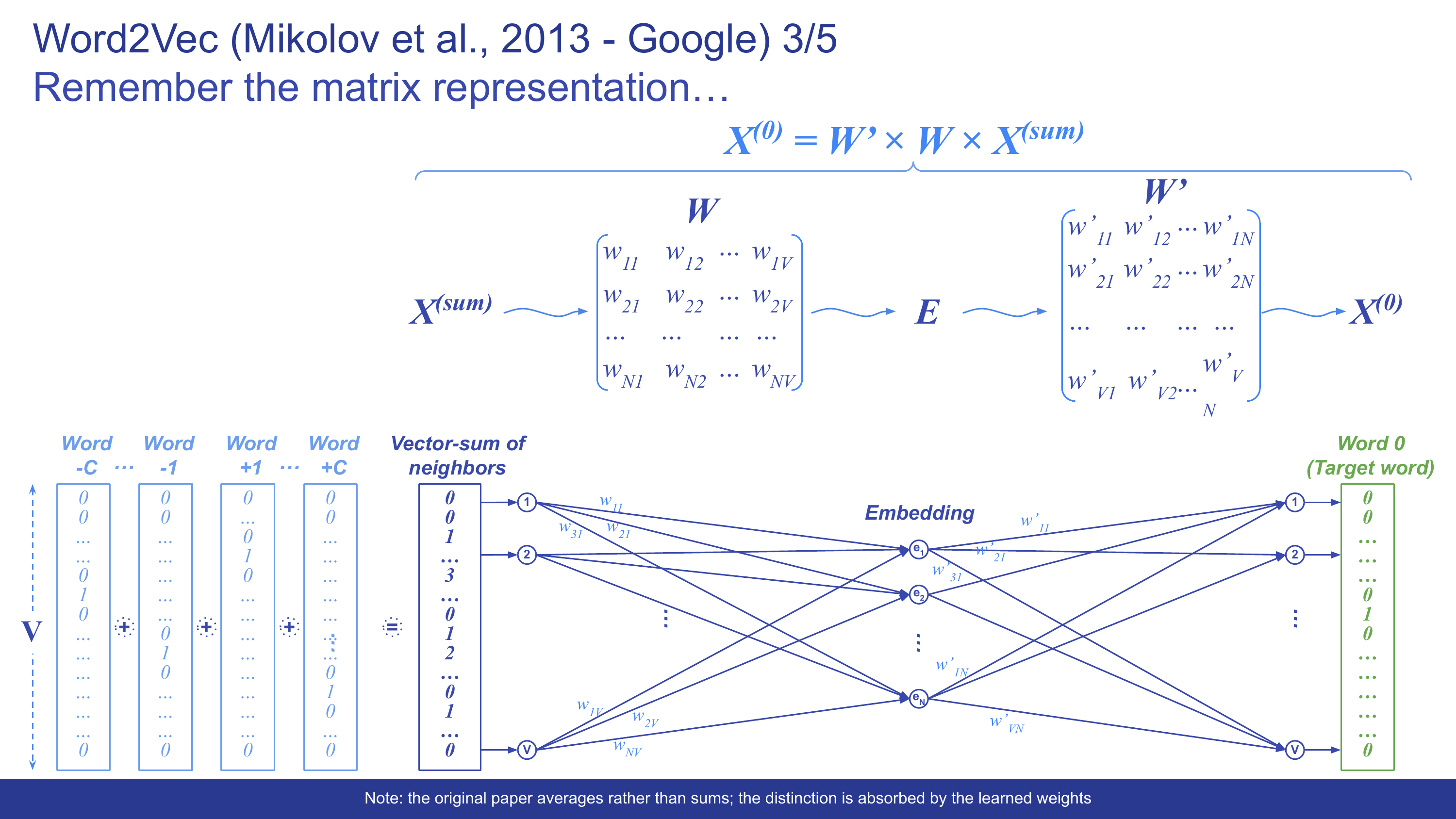
As in chapter 7, it’s convenient to write the whole thing compactly: X(0) = W’ × W × X(sum). The sum of the context vectors passes through matrix W to produce the hidden layer E, then passes through matrix W’ to produce the prediction X(0). Two matrix multiplications, exactly as in the two-layer example of chapter 7.
Here comes the touch that makes Word2Vec truly practical: no human labeling is needed at all. You take any text — a novel, an article, all of Wikipedia — and slide a window across it: every position of the window generates a context/target pair by itself. A sentence like In York Abbey, a wooden abacus from the 1700s was discovered automatically produces a dozen or so training examples, simply by moving the window one word at a time. It’s the same trick behind the self-supervised pre-training we met in chapter 5: raw text labels itself.
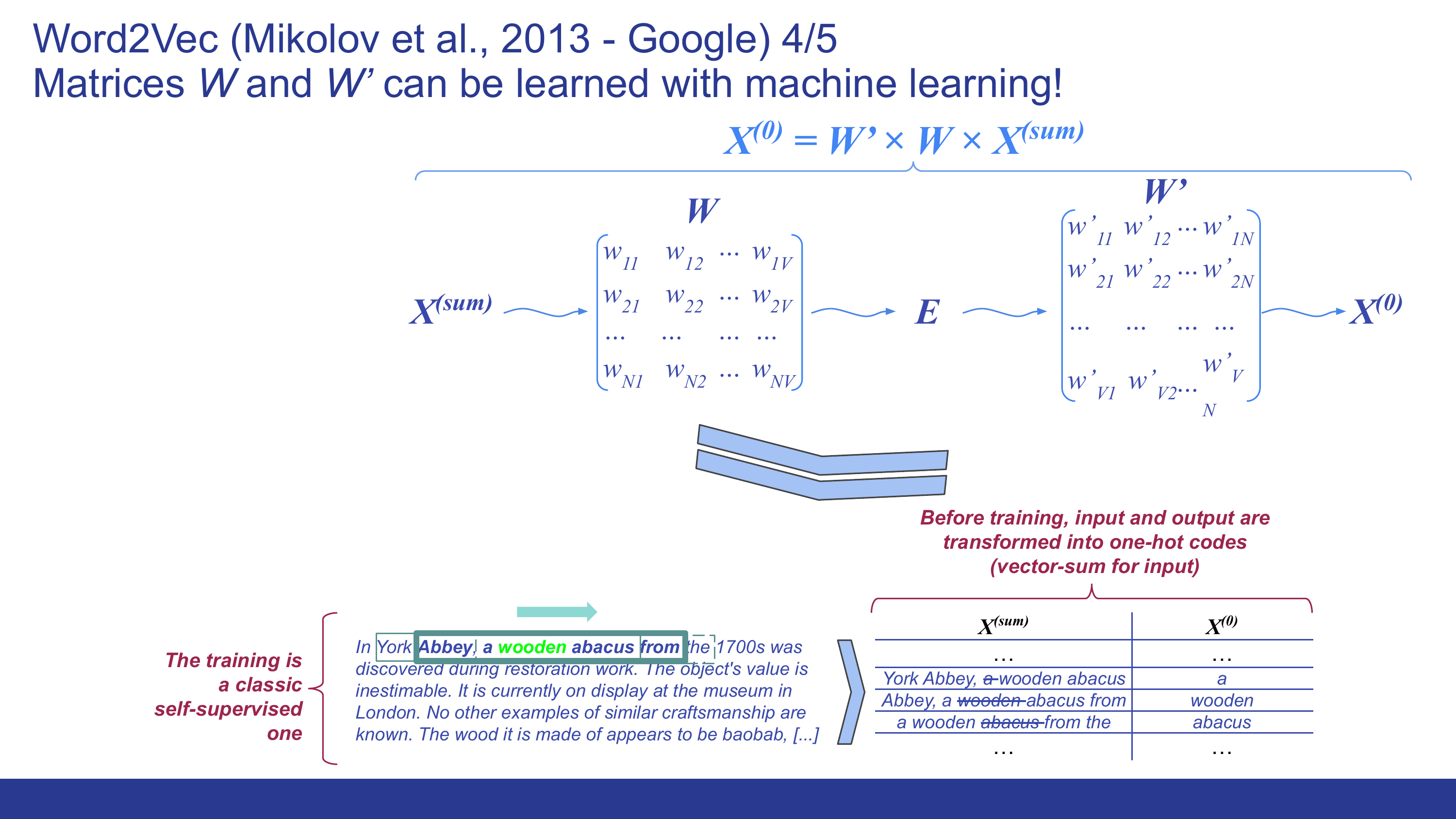
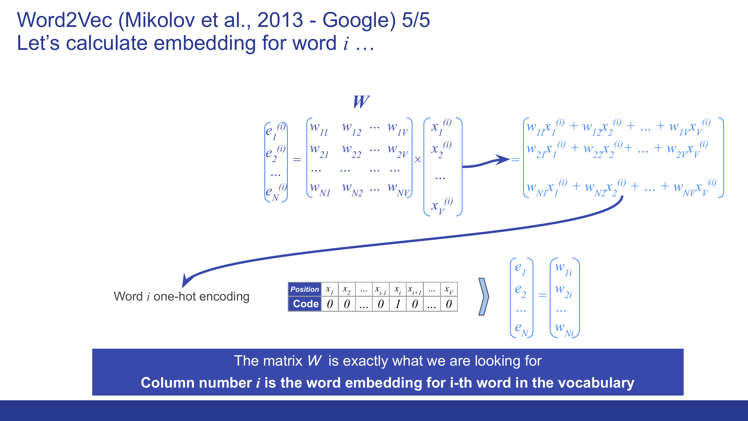
Matrices W and W’ are trained with ordinary backpropagation from chapter 8, minimizing the prediction error on the target word across millions of examples. But the real result of all this work isn’t the prediction itself, but a byproduct of the process. Once training is finished, column i of matrix W is exactly the embedding vector for the i-th word in the vocabulary. The hidden layer, the one we called E, turns out to be nothing other than the dense space we’d been looking for since chapter 11 — and the meaning of its dimensions was chosen by no one: training found it on its own, by looking at which contexts each word appears in, and there’s no guarantee it’s a meaning a human could actually grasp.
A vector representation obtained this way achieves exactly what we set out to do back in chapter 11: a space in which closeness of meaning — here, between a word and the words around it — translates into geometric closeness. These spaces, though, also hide surprising properties and limitations, which we’ll see in chapter 13.